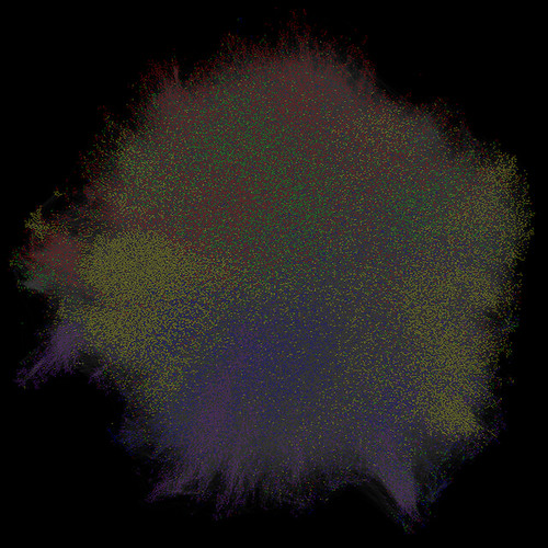
I'm pretty proud of this, which I produced during Twitter's most recent hackweek:
It's a map of verified users of Twitter. The layout is calculated according to the mutual follow graph connecting these users, ie. relationships where @x follows @y and @y follows @x. The coloring is determined by user category (eg. sport, music, etc).
The Twitter Media blog post has some good information about how to think about the visual and what we can deduce from it; what follow here are the gory details behind how it was built—for data visualization dilettantes and cargo-culters like myself.
What on earth
First of all: what exactly is this thing? In technical terms it's a force-directed layout of the largest connected component of the verified user mutual follow graph. That single large connected component happens to contain over 99% of verified users; a handful are off on islands of their own, not connected to this clown hairball by mutual follows, and they're not shown.
How it came to be
Here's how it looked at the beginning of hackweek; this is a first quick pass at the force-directed layout of a random sample of verified users:
(More detail below on the tools that I used to make this image but for those already wondering, the hard work was done by Graphviz, specifically sfdp and neato)first render of the largest connected component of the graph of mutual follows amongst verified users #hackweekpic.twitter.com/wklPDFY0zv
— Isaac Hepworth (@isaach) July 9, 2013
This was looking promising (and attractive in its own way, I thought) but as I added more and more users it just became a big dense white blob with no apparent structure. I figured I'd have a go at coloring the nodes by user category (sports, music, news, and so on) to see if some structure would reveal.
I started off by just highlighting TV-related accounts, which you can see in this graph of a 10% sample:
and this showed enough promise to add colors for other high-level categories.

I liked the way colors clustered together, but now my diagram was looking a bit drab:
The density of the gray edges was just sucking the saturation out—and their uniformity was obscuring further structure, I figured.
So I colored the edges: any edge connecting two nodes of the same color would be colored accordingly: a yellow line to connect two sports people following each other; a red line to connect two musicians following each other; and so on.
Now the clusters were really clear. I liked this a lot, and I rendered a really large version:
spent the weekend rendering a gigapixel version of this bad boy: a graph of verified users on twitter. #hackweekendpic.twitter.com/rzQ1fWYUZy
— Isaac Hepworth (@isaach) July 15, 2013
The result is what you see in the Twitter Media blog post. Not quite a gigapixel, but near enough.
The generation process in detail
Obviously, the process starts by capturing the follow relationships between verified users on Twitter. You can do this yourself easily enough using the Twitter API:
- find verified users by looking at who @verified follows;
- for each, find who they follow;
- filter this dataset down to mutual follows.
screen_name_1 [tab] screen_name_2

screen_name_1 [tab] screen_name_3

screen_name_4 [tab] screen_name_5
Once you have this you can use your favorite awk or perl or bash one-liners to turn this into a bare graph in DOT format:
digraph my_graph {

    screen_name_1 -> screen_name_2

    screen_name_1 -> screen_name_3

    screen_name_4 -> screen_name_5

}
At this point I used Graphviz's comps utility to extract the largest connected component of the graph:
cat graph.gv | ccomps -zX#0 > graph-cc0.gv
Now we have the core data of interest in graph-cc0.gv and we can iterate on the following:
- layout: I used sfdp to produce a force-directed layout of the graph;
- coloring: I wrote a handful of lines of Python to color the laid-out graph according to the category of user;
- rasterization: I used neato to render the graph to a PNG.
- presentation: I uploaded to zoom.it to share the result.
I used a MacBook Air to do this work. Step (1) typically took a few minutes, (2) was 20 seconds or so; (3) was 10–120 minutes depending on the output size; (4) was actually the slowest step—a few days to process and present the final version. The graphviz tools are single-threaded and tend to be CPU-bound; you can get some wins with better hardware on (3), but only very modest ones.
Here's how it all adds up into a single script:
No comments:
Post a Comment